

Math Behind Backpropagation and Gradient Descent
Learn how Neural Networks are trained under the hood...


So, you're ready to dive into the Math stuff behind neural networks (NNs)? Lucky you! You've come to the right place!
Yet, before you begin, make sure that you meet the following prerequisites
Linear algebra
Advanced differentiation (especially, the chain rule)
How a Neural Network works (read this)
🪜 Gradient Descent From the Ground Up
The purpose of Gradient Descent is to optimise the independent variables (e.g. weights and biases in an NN) of a function to reach the least possible cost for given training examples.
Let's break it down!
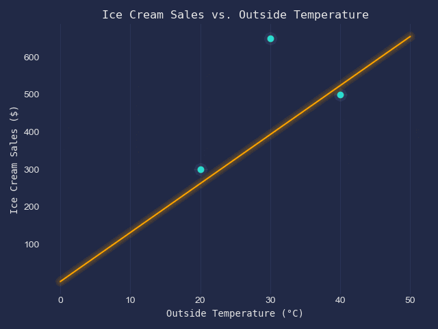
We have got the following table of data.
| x - Outside Temperature (°C) | y - Ice Scream Sales ($) |
| 20 | 300 |
| 30 | 650 |
| 40 | 500 |
When displayed on a scatter plot, they look like this;

Our goal is to fit a line of best fit into this scatter plot.
Firstly, let's define the equation of a line,
$$y = mx+c$$
m is the slope and c is the intercept (these are the parameters we can directly adjust)
We are going to use Gradient Descent to calculate the optimal values for the intercept and the slope.
For the cost function, let's use squared error. Thus, the cost function of the line can be defined as,
$$C = (300-y_1)^2+(650-y_2)^2+(500-y_3)^2$$
y-values represent the prediction of the model for the corresponding x-coordinates.
The expanded version after substituting the x-coordinates,
$$C = [300-(20m+c)]^2+[650-(30m+c)]^2+[500-(40m+c)]^2$$
We differentiate the cost function with respect to every parameter we have. In this case, we have only 2 parameters: intercept (c) and slope (m).
So, these are the derivatives we get after differentiating using the chain rule,
$$\frac{dC}{dm} = -40(300-20m-c)-60(650-30m-c)-80(500-40m-c)$$
$$\frac{dC}{dc} = -2(300-20m-c)-2(650-30m-c)-2(500-40m-c)$$
Initially, we pick random values for intercept and slope.
To keep things simpler, we'll assume we started with,
$$m=1 \ \& \ c=0$$
Using the current variables, we calculate the gradient of the cost function at the given slope/intercept,
$$\frac{dC}{dm} = -40(300-20)-60(650-30)-80(500-40) = -85200$$
$$\frac{dC}{dc} = -2(300-20)-2(650-30)-2(500-40) = -2720$$
We change the independent variable (slope/intercept) by a value called the step size. We calculate it as a percentage of the gradient we calculated above. This percentage is called the Learning Rate. It is constant and is defined when creating the model (thus, it is a hyperparameter).
In our case, we'll say the learning rate is 0.01 (1%).
Based on that, the step sizes for our variables are,
$$\text{Slope's Step Size} = -82200 \times 0.1 = -852$$
$$\text{Intercept's Step Size} = -2620 \times 0.1 = -27.2$$
We normally subtract these from the current variable value to get a new value. That's because we are trying to reach a minimum of the cost function.

This is similar yet more complex for higher dimensions... That requires enough knowledge about Multi-Variable Calculus.
Anyways, based on these facts, our new slope and intercept are,
$$\text{New Slope} = \text{Current Slope} - \text{Slope's Step Size} = 1-(-852) = 853$$
$$\text{New Intercept} = \text{Current} - \text{Intercepts' Step Size} = 0 - (-27.2) = 27.2$$
Obviously, these aren't the best values ever. That's why this process is iterated a considerable number of times. Once the improvement becomes negligible, the gradient descent algorithm stops.
Alright, if you are math savvy, you may be questioning why the heck we iteratively do this when we could simply calculate the optimal values by making their derivatives equal to 0.
Of course, we can find the turning points of a function that way. Yet for higher dimensions (like 100,000+), simplifying an equation becomes utterly complex due to the huge number of independent variables that exist.
🔗 GD's Connection to Backpropagation
Now, you know how gradient descent works. Yet, how is it used to tweak the weights and biases of a neural network?
If you have a fundamental understanding of how Neural Networks work, you may recall that we calculate the required proportional changes. Then, we propagate them backwards through the NN since output layer activations depend on preceding layer activations.
To be frank, that's just a human-comprehensible way to describe Gradient Descent's role in tweaking parameters. Those proportional changes are merely the step sizes for each weight and bias calculated through gradient descent.
Let's take an example of a neural network which has 3 layers with one neuron in each.

We perform backpropagation after forward feeding the inputs. So, remember that we already have the activations for each neuron.
To begin with, we calculate the cost of the whole NN. Using squared error, we get the cost,
$$C = (d - a_3)^2$$
let d = desired output
We know the output layer activations depend on the following factors,
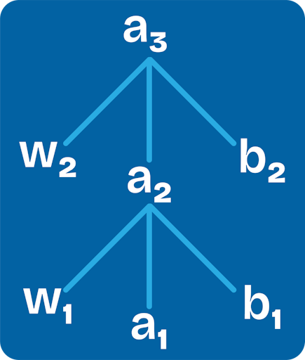
$$a_3 = (w_2 \times a_2 + b_2)$$
So, we can do the following 3 options to tweak the last neuron activation. That way, we can approach d (desired value) and minimise the cost function.
Change the weight (w2)
Change the bias (b2)
Change the activation (a2)
We calculate the derivative of the cost function with respect to every variable.
$$\frac{dC}{dw_2} = -2a_2(d-w_2\times a_2 - b_2)$$
$$\frac{dC}{db_2} = -2(d-w_2\times a_2 - b_2)$$
So far, we can directly influence the weights and biases by subtracting the step size we calculate using gradient descent (like previously).
Yet, the last layer activation/s (a2, in this case) can't be modified in that way. That's because they depend on their weighted sum and the bias. So they are even influenced by the previous layer's activations;
$$a_2 = w_1 \times a_1+b_1$$
To keep things simple, let's calculate the derivative of the cost function with respect to a2,
$$\frac{dC}{da_2} = -2w_2(d-w_2\times a_2 - b_2)$$
This is where things get interesting. Since we have successfully calculated the step sizes for w2 and b2, we are unfolding a2 by substituting the below function,
$$a_2 = a_1 \times w_1 + b_1$$
Similarly, we calculate the required step sizes for every weight and bias (w_2, b_2).
That's how we go deeper, layer by layer! This is why it is called Backpropagation. We calculate the step sizes for every weight and bias of the NN this way.
In fact, these step sizes are different from one training example to another.
So, we find the average step size for every weight and bias based on all the training examples we have. Then, we make those changes through subtraction :)
This way, over many training epochs, the weights and biases become closer to the minimum!
📦 Stochastic Gradient Descent (SGD)
Gradient descent is computationally slow as it is performed for every training example.
Stochastic Gradient Descent kicks in to solve this problem.
Here, instead of performing gradient descent for every training example in an epoch, it is only performed for one or a specific number (mini-batch) of randomly selected training examples.
The mini-batch size is a constant value that is set when initialising the NN.
That's it!
👋 Conclusion
Yay, now you have an intuitive understanding of how NNs are trained.
If you were able to get this far, go ahead and give yourself a treat because you just burst your mind through various layers of complexity!
Don't worry if it takes time for your brain to grasp all these.
🤞 All the best! You've got this!